Why DCT is good for image coding?

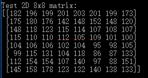
In my last post, I use real image block data to test the DCT transform. Using this data, we can check the advantage of using DCT for image coding. Here is our first test data.

By following code, we can get the inverse result of DCT transform.

[code lang=“python”] # inverse transform, calculate the S by coefficients & basis S_inverse = np.zeros([N, N]) for k in range(0, 2): for j in range(0, 2): S_inverse = S_inverse + T[k][j]*U[k][j] [/code]

We can change variable N in above code to get the influence of low or high frequency coefficients. And we use PSNR to check the difference between origin test data and inverse result.

[code lang=“python”] def psnr(img1, img2): mse = np.mean(np.square(img1 - img2)) if mse == 0: return 100 PIXEL_MAX = 255.0 return 10 * math.log10(PIXEL_MAX**2 / mse) [/code]

Here is the PSNR result by changing N in inverse transform.

The PSNR above 40~45 can be regarded as good as enough to see any difference in human eyes.

And we can use a whole image as input to check the PSNR result. I use famous Lena’s 512x512 picture as test data. I also provide two ways to calculate the image forward and inverse transform. One way is using SciPy embeded function and the other way is using my own basis patterns function which you can find in my last post.

Here is the main process of the program.

[code lang=“python”] im = plt.imread(“lena2.tif”).astype(float) print(im.shape) #dct, img_dct = ImgDctUsingScipy(im) # using Scipy way dct, img_dct = ImgDctUsingDetail(im) # using my own calculation way

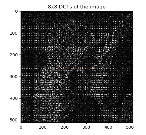
plt.figure() plt.imshow(dct,cmap=‘gray’,vmax = np.max(dct)*0.01,vmin = 0) plt.title( “8x8 DCTs of the image”)

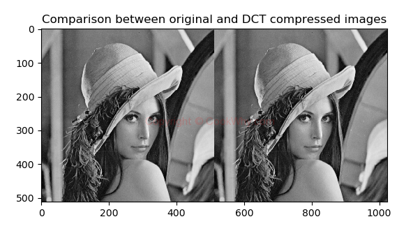
plt.figure() plt.imshow( np.hstack( (im, img_dct) ) ,cmap=‘gray’) plt.title(“Comparison between original and DCT compressed images” )

diff = psnr(im, img_dct) print("\nPSNR is: “, np.around(diff, 2))

plt.show() [/code]

The function ImgDctUsingScipy and ImgDctUsingDetail are two ways to calculate the forward and inverse transform. Using ImgDctUsingScipy as example, the function is very simple.

[code lang=“python”] def ImgDctUsingScipy(im): imsize = im.shape dct = np.zeros(imsize) for i in r_[:imsize[0]:8]: for j in r_[:imsize[1]:8]: dct[i:(i+8),j:(j+8)] = img2dct( im[i:(i+8),j:(j+8)] )

#get the inverse image img_dct = np.zeros(imsize) for i in r_[:imsize[0]:8]: for j in r_[:imsize[1]:8]: img_dct[i:(i+8),j:(j+8)] = dct2img( dct[i:(i+8),j:(j+8)] )

return dct, np.round(img_dct, 0) [/code]

After running the program, We will get following three pictures, and we can see the original and reversed image is the same.

If we change the N in step N, we will get different PSNR value.

And the visual result of these four coefficients selection is as below.

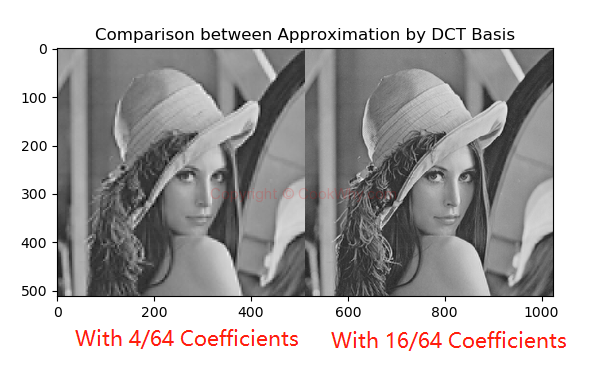
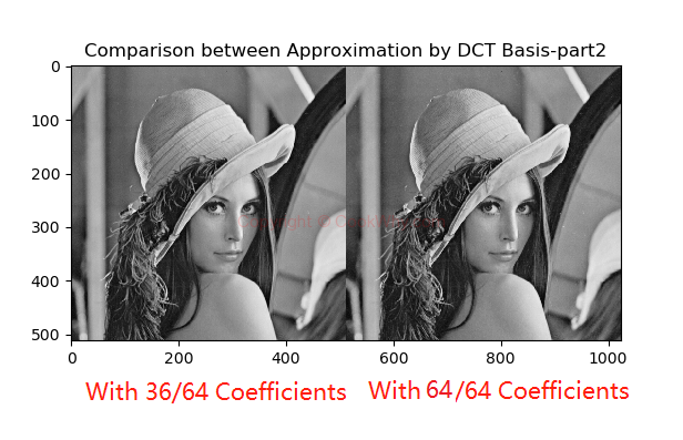
We can see that with 64/64, the image quality is almost as the original one. In fact, with the 36/64 coefficients, the quality is also good enough for common compression usage.

That’s why DCT is good for image coding!